Balmer series — LineProfile class
Script: examples/example_balmer_lineprofile.py
Computes Hα through Hε at DIII-D-like edge conditions (B = 12 T,
\(N_e = 10^{21}\) m-3, \(T_e = 1\) eV, \(T_i = 10\) eV) using
the LineProfile class. Each panel shows:
Transverse (90°) and parallel (0°) broadened profiles
Discrete stick spectrum at zero microfield (\(F = 0\))
Ti_ev is supplied so the static solver folds in thermal Doppler
broadening — without it the Stark-Zeeman components at these conditions are
narrower than the grid spacing, and the profile comes out as an
undersampled, spiky Lorentzian sum rather than a smooth curve.
Each line’s wavelength window is set individually rather than sharing one fixed half-width: Stark broadening grows rapidly with \(n\), so a window sized for Hα would truncate the wings of Hδ or Hε — at a fixed ±1 nm window the profile is still at 6 % of its peak at the edge for Hε versus 0.4 % for Hα — showing up as an apparently “clipped” profile that never reaches zero. Each half-window below is instead sized so its own line has decayed to <0.2 % of peak by the panel edge.
Code
  1#!/usr/bin/env python3
  2"""
  3Balmer series (Hα – Hε) at DIII-D-like edge conditions
  4B = 12 T,  Ne = 1e21 m⁻³,  Te = Ti = 10 eV  —  transverse observation
  5
  6Ti_ev is supplied so the static solver folds in thermal Doppler broadening
  7(the compute_static_profile default is a bare, un-Dopplered profile). Without
  8it, the natural/electron-impact linewidth at these conditions is narrower
  9than the wavelength-grid spacing, and the resulting undersampled Lorentzians
 10show up as spiky, sawtooth-textured curves rather than the smooth envelope a
 11real (Doppler-broadened) spectrum would have.
 12"""
 13
 14import numpy as np
 15import matplotlib.pyplot as plt
 16import sys, os
 17
 18sys.path.insert(0, os.path.abspath(os.path.join(os.path.dirname(__file__), "..")))
 19
 20from starkzee.line_profile import LineProfile
 21
 22# ── Plasma conditions ─────────────────────────────────────────────────────────
 23Z   = 1
 24B   = 12.0   # T
 25Ne  = 1e21   # m⁻³
 26Te  = 1.0    # eV
 27Ti  = 10.0   # eV (Doppler; see module docstring)
 28
 29# (n_u, n_l, label, half-window [nm])
 30# Stark broadening grows rapidly with n, so a fixed half-window truncates the
 31# wings of the higher lines instead of letting them decay to ~0 (at a fixed
 32# 1.0 nm window, the profile is still at 6% of its peak at the edge for Hε
 33# vs 0.4% for Hα) -- each half-window below is sized so its line's profile
 34# has decayed to <0.2% of peak by the edge.
 35LINES = [
 36    (3, 2, "Hα", 1.75),
 37    (4, 2, "Hβ", 2.00),
 38    (5, 2, "Hγ", 2.50),
 39    (6, 2, "Hδ", 3.50),
 40    (7, 2, "Hε", 5.00),
 41]
 42
 43PROFILE_KWARGS = dict(
 44    num_f=30, num_mu=8,
 45    quadratic_zeeman=False,
 46    fine_structure=False,
 47    frequency_dependent_width=False,
 48)
 49
 50# ── Compute ───────────────────────────────────────────────────────────────────
 51profiles = {}
 52for n_u, n_l, label, hw_nm in LINES:
 53    lp = LineProfile(n_u=n_u, n_l=n_l, B=B, Ne_m3=Ne, Te_ev=Te, Ti_ev=Ti, species='H')
 54
 55    wl_grid = np.linspace(lp.E0_wavelength_nm - hw_nm, lp.E0_wavelength_nm + hw_nm, 1000)
 56    print(f"Computing {label} (n={n_u}→{n_l}), λ₀={lp.E0_wavelength_nm:.2f} nm …", flush=True)
 57
 58    lp.compute_profile(wl_grid, grid_type='wavelength_nm', **PROFILE_KWARGS)
 59    lp.compute_discrete(Fz=0.0, Fx=0.0, quadratic_zeeman=False)
 60    profiles[label] = lp
 61    print(f"  → {len(lp.discrete.energy_ev)} discrete transitions", flush=True)
 62
 63# ── Plot ──────────────────────────────────────────────────────────────────────
 64fig, axes = plt.subplots(len(LINES), 1, figsize=(10, 9), sharex=False)
 65fig.suptitle(
 66    rf"Balmer series — Stark-Zeeman  |  B = {B} T,  "
 67    rf"$N_e$ = {Ne:.0e} m$^{{-3}}$,  $T_e$ = {Te} eV,  $T_i$ = {Ti} eV",
 68    fontsize=12,
 69)
 70
 71COLORS_Q = {0: "black", 1: "C3", -1: "C2"}
 72LABELS_Q  = {0: "π", 1: "σ+", -1: "σ−"}
 73
 74for ax, (n_u, n_l, label, _) in zip(axes, LINES):
 75    lp   = profiles[label]
 76    disc = lp.discrete
 77
 78    # Broadened profiles — normalize to peak transverse intensity
 79    peak = lp.profile_transverse.max() or 1.0
 80    ax.plot(lp.detuning_nm, lp.profile_transverse / peak,
 81            color="C0", lw=1.8, label="Transverse (90°)")
 82    ax.plot(lp.detuning_nm, lp.profile_parallel / peak,
 83            color="C1", lw=1.2, ls="--", label="Parallel (0°)")
 84
 85    # Stick spectrum at zero microfield
 86    max_s = disc.strength.max() or 1.0
 87    drawn = set()
 88    for dλ, q, s in zip(disc.detuning_nm, disc.q, disc.strength):
 89        kw = dict(color=COLORS_Q[int(q)], lw=1.0, alpha=0.6)
 90        if int(q) not in drawn:
 91            kw["label"] = LABELS_Q[int(q)]
 92            drawn.add(int(q))
 93        ax.axvline(dλ, ymin=0, ymax=s / max_s * 0.35, **kw)
 94
 95    ax.set_xlim(lp.detuning_nm.min(), lp.detuning_nm.max())
 96    ax.set_ylim(bottom=0)
 97    ax.set_title(rf"{label}  ($n={n_u}\to{n_l}$,  $\lambda_0={lp.E0_wavelength_nm:.2f}$ nm)",
 98                 fontsize=10)
 99    ax.set_ylabel("Norm. intensity", fontsize=9)
100    ax.legend(fontsize=7, loc="upper right", ncol=2)
101    ax.grid(True, alpha=0.3)
102
103axes[-1].set_xlabel(r"$\lambda - \lambda_0$  (nm)", fontsize=11)
104
105plt.tight_layout()
106out = "example_balmer_lineprofile.png"
107plt.savefig(out, dpi=150, bbox_inches="tight")
108print(f"\nSaved {out}")
109plt.show()
Result
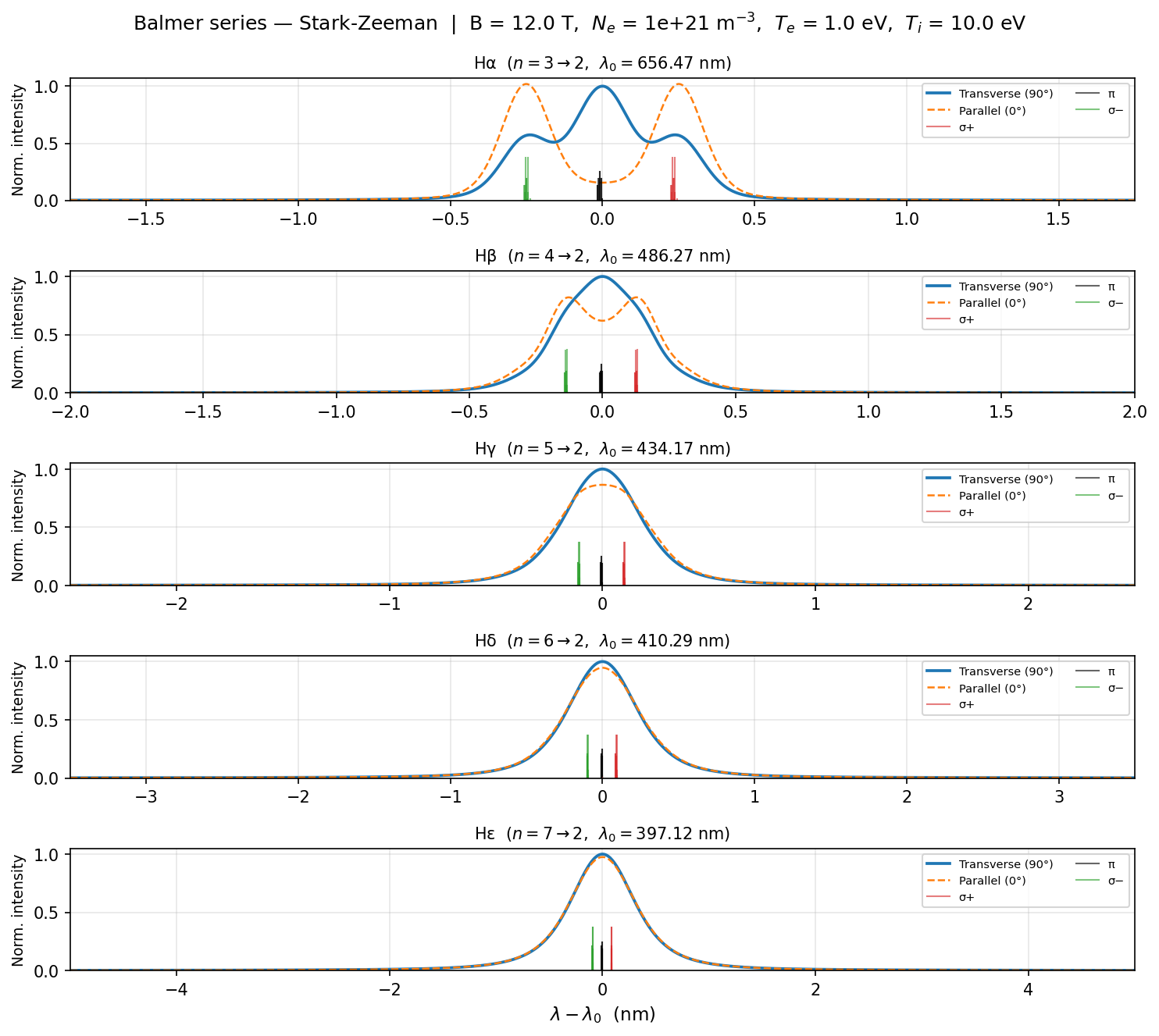
Transverse and parallel broadened profiles with the zero-field stick spectrum overlaid, for Hα through Hε.