Lyman-α at high B
Three scripts computing H Lyman-α (n=2→1) at increasing magnetic field — 100 T, 500 T, and 1000 T — exploring the transition from the intermediate-field to the Paschen-Back regime. Conditions are \(N_e = 5\times10^{25}\) m-3, \(T_e = 100\) eV throughout, with no Doppler or instrumental convolution (pure Stark-Zeeman profile). Each script’s title is loosely inspired by Figure 3 of Ferri, Peyrusse & Calisti (2022) — note that figure was computed for C VI (Z = 6), not H; these scripts use H (Z = 1), so absolute splittings and widths differ from the published figure.
B = 100 T (test_lyman_alpha.py)
  1#!/usr/bin/env python3
  2"""
  3H Lyman-alpha Stark-Zeeman Splitting at B = 100 T
  4
  5Illustrates the polarization structure of Lyman-alpha (n=2 -> n=1) under
  6plasma conditions loosely inspired by the Figure 3 benchmark of Ferri,
  7Peyrusse & Calisti (2022, DOI: 10.1063/5.0058552) — note that figure was
  8computed for C VI (Z = 6), not H; this script uses H (Z = 1) throughout, so
  9absolute splittings and widths differ from the published figure.
 10
 11Conditions:
 12  - Radiator: H (Z = 1), Lyman-alpha (n=2 -> n=1)
 13  - B = 100 T
 14  - Ne = 5e25 m^-3
 15  - Te = 100 eV
 16  - No Doppler or instrumental convolution (pure Stark-Zeeman profile)
 17
 18The pi component is multiplied by -1 for visual separation of polarizations.
 19The x-axis is energy detuning (eV) from the unperturbed transition center E0.
 20"""
 21
 22import os
 23import sys
 24import numpy as np
 25import matplotlib.pyplot as plt
 26
 27# Ensure starkzee package is in path
 28sys.path.insert(0, os.path.abspath(os.path.join(os.path.dirname(__file__), "..")))
 29
 30from starkzee.utils import energy_ev_to_wavelength_nm, RYDBERG_EV
 31from starkzee.static_profile import calculate_static_profile
 32
 33
 34def run_lyman_alpha_test():
 35    # ── Physical parameters (loosely inspired by paper Fig. 3, but H not C VI) ─
 36    Z  = 1        # Hydrogen
 37    B  = 100.0    # Tesla
 38    Ne = 5e25     # m^-3
 39    Te = 100.0    # eV
 40
 41    # Unperturbed Lyman-alpha transition energy for H: n=2 -> n=1
 42    E_upper = -(Z**2) * RYDBERG_EV / 4.0   # n=2 level
 43    E_lower = -(Z**2) * RYDBERG_EV          # n=1 level
 44    E0 = E_upper - E_lower                  # ~10.2 eV for H
 45
 46    # Energy grid: ±0.20 eV around E0
 47    detuning_grid = np.linspace(-0.2, 0.2, 500)
 48    energies_ev   = E0 + detuning_grid
 49
 50    print("=" * 70)
 51    print("test_lyman_alpha: H Lyman-alpha Stark-Zeeman at B = 100 T")
 52    print(f"  Z={Z}, B={B} T, Ne={Ne:.1e} m^-3, Te={Te} eV")
 53    print(f"  Unperturbed center E0 = {E0:.6f} eV  "
 54          f"({energy_ev_to_wavelength_nm(E0):.6f} nm)")
 55    print("=" * 70)
 56
 57    # ── Compute static (unconvolved) Stark-Zeeman profile ──────────────────
 58    print("-> Computing static Stark-Zeeman profile (unconvolved)…")
 59    pi, sig_plus, sig_minus = calculate_static_profile(
 60        n_u=2, n_l=1, Z=Z, B=B, Ne_m3=Ne, Te_ev=Te,
 61        energies_ev=energies_ev,
 62        num_f=30, num_mu=10,
 63        use_screening=True,
 64        quadratic_zeeman=True,
 65        frequency_dependent_width=True,
 66    )
 67
 68    # ── Plot — Figure 3 layout ──────────────────────────────────────────────
 69    fig, ax = plt.subplots(figsize=(9, 6))
 70
 71    ax.plot(detuning_grid, sig_plus,  color='#10b981', linewidth=2.2,
 72            label=r'$\sigma_+$  ($q = +1$)')
 73    ax.plot(detuning_grid, sig_minus, color='#f59e0b', linewidth=2.2,
 74            label=r'$\sigma_-$  ($q = -1$)')
 75    ax.plot(detuning_grid, -pi,       color='#ef4444', linewidth=2.2,
 76            linestyle='--', label=r'$-\pi$  ($q = 0$)')
 77
 78    ax.axhline(0, color='gray', linestyle=':', linewidth=0.9)
 79    ax.axvline(0, color='gray', linestyle='--', linewidth=0.8, alpha=0.6,
 80               label=f'$E_0 = {E0:.4f}$ eV')
 81
 82    ax.set_title(
 83        f"SZ Lyman-$\\alpha$ of H  (B = {B:.0f} T, "
 84        f"$N_e = {Ne:.0e}$ m$^{{-3}}$, $T_e = {Te:.0f}$ eV)\n"
 85        r"Pure Stark-Zeeman profile",
 86        fontsize=12, pad=12,
 87    )
 88    ax.set_xlabel(r"Energy detuning from $E_0$ (eV)", fontsize=11)
 89    ax.set_ylabel("Intensity (arb. units)", fontsize=11)
 90    ax.set_xlim(-0.2, 0.2)
 91
 92    ax.grid(True, linestyle=':', alpha=0.55)
 93    ax.legend(frameon=True, fontsize=10)
 94
 95    plt.tight_layout()
 96    plot_file = os.path.join(os.path.dirname(__file__), "lyman_alpha_100T.png")
 97    plt.savefig(plot_file, dpi=300)
 98    print(f"Plot saved → {plot_file}")
 99    plt.show()
100
101
102if __name__ == "__main__":
103    run_lyman_alpha_test()
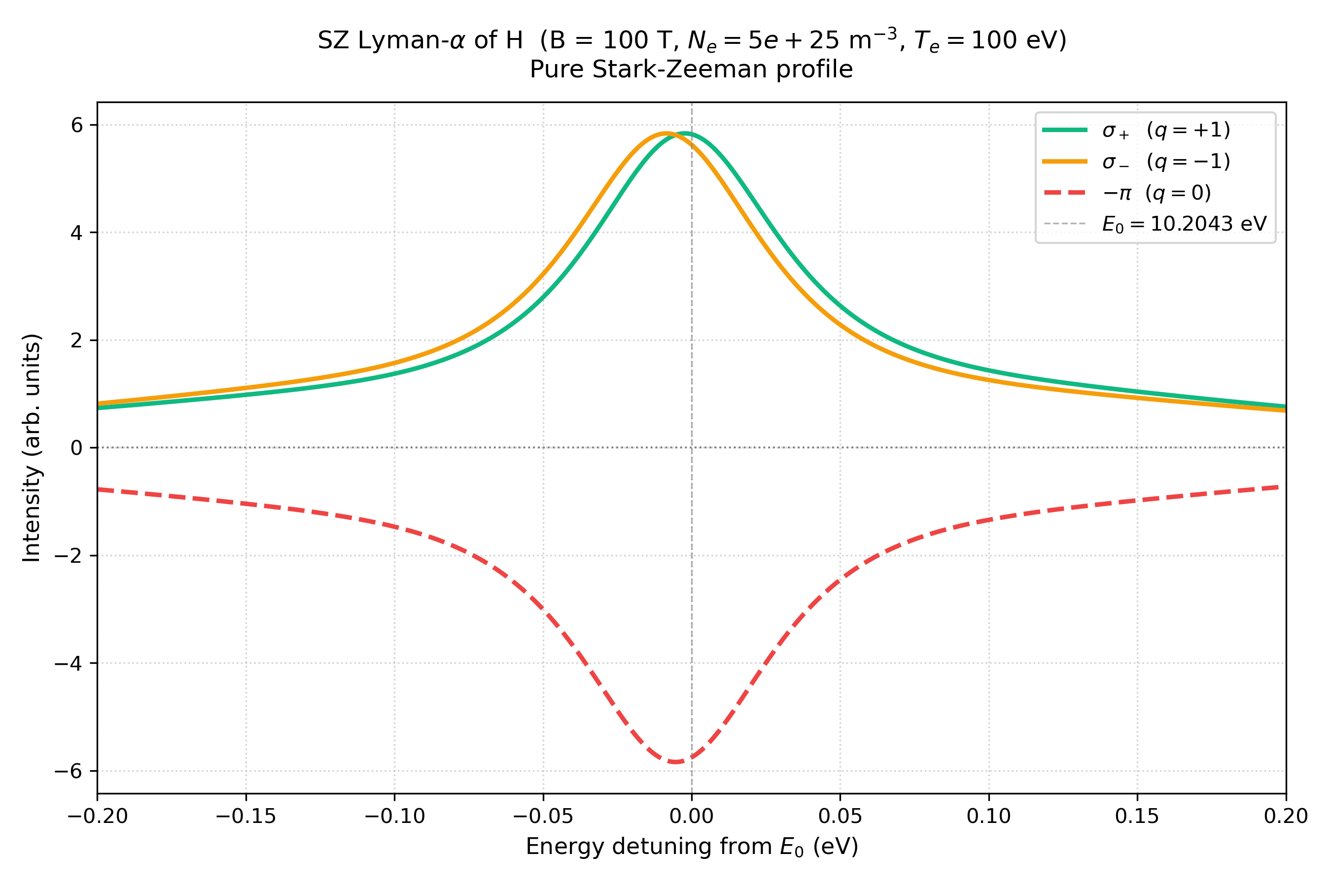
π, σ+, σ− components of H Ly-α at B = 100 T (π shown inverted for visual separation).
B = 500 T (test_lyman_alpha_500T.py)
 1#!/usr/bin/env python3
 2"""
 3H Lyman-alpha Stark-Zeeman Splitting at B = 500 T
 4
 5Higher-field companion to test_lyman_alpha.py (100 T), loosely inspired by
 6the Figure 3 benchmark of Ferri, Peyrusse & Calisti (2022,
 7DOI: 10.1063/5.0058552) — that figure used C VI (Z = 6); this script uses
 8H (Z = 1) throughout.
 9
10Conditions:
11  - Radiator: H (Z = 1), Lyman-alpha (n=2 → n=1)
12  - B = 500 T
13  - Ne = 5e25 m^-3
14  - Te = 100 eV
15  - No convolution (pure Stark-Zeeman profile)
16
17Energy range ±0.20 eV around E0.  The pi component is multiplied by -1 for
18visual separation of polarizations.
19"""
20
21import os
22import sys
23import numpy as np
24import matplotlib.pyplot as plt
25
26sys.path.insert(0, os.path.abspath(os.path.join(os.path.dirname(__file__), "..")))
27
28from starkzee.utils import energy_ev_to_wavelength_nm, RYDBERG_EV
29from starkzee.static_profile import calculate_static_profile
30
31
32def run_test():
33    # ── Physical parameters ────────────────────────────────────────────────
34    Z  = 1        # Hydrogen
35    B  = 500.0    # Tesla
36    Ne = 5e25     # m^-3
37    Te = 100.0    # eV
38
39    # Unperturbed Lyman-alpha for H (n=2 → n=1)
40    E0 = (Z**2) * RYDBERG_EV * (1.0 - 1.0/4.0)   # = (3/4) Z² Ry
41
42    # Energy grid: ±0.20 eV around E0
43    detuning_grid = np.linspace(-0.2, 0.2, 600)
44    energies_ev   = E0 + detuning_grid
45
46    print("=" * 70)
47    print("test_lyman_alpha_500T: H Lyman-alpha — B = 500 T")
48    print(f"  Z={Z}, B={B} T, Ne={Ne:.1e} m^-3, Te={Te} eV")
49    print(f"  E0 = {E0:.6f} eV  ({energy_ev_to_wavelength_nm(E0):.6f} nm)")
50    print("=" * 70)
51
52    print("-> Computing static Stark-Zeeman profile (unconvolved)…")
53    pi, sig_plus, sig_minus = calculate_static_profile(
54        n_u=2, n_l=1, Z=Z, B=B, Ne_m3=Ne, Te_ev=Te,
55        energies_ev=energies_ev,
56        num_f=30, num_mu=10,
57        use_screening=True,
58        quadratic_zeeman=True,
59        frequency_dependent_width=True,
60    )
61
62    # ── Plot ───────────────────────────────────────────────────────────────
63    fig, ax = plt.subplots(figsize=(9, 6))
64
65    ax.plot(detuning_grid, sig_plus,  color='#10b981', linewidth=2.2,
66            label=r'$\sigma_+$  ($q = +1$)')
67    ax.plot(detuning_grid, sig_minus, color='#f59e0b', linewidth=2.2,
68            label=r'$\sigma_-$  ($q = -1$)')
69    ax.plot(detuning_grid, -pi,       color='#ef4444', linewidth=2.2,
70            linestyle='--', label=r'$-\pi$  ($q = 0$)')
71
72    ax.axhline(0, color='gray', linestyle=':', linewidth=0.9)
73    ax.axvline(0, color='gray', linestyle='--', linewidth=0.8, alpha=0.6,
74               label=f'$E_0 = {E0:.4f}$ eV')
75
76    ax.set_title(
77        f"SZ Lyman-$\\alpha$ of H  (B = {B:.0f} T, "
78        f"$N_e = {Ne:.0e}$ m$^{{-3}}$, $T_e = {Te:.0f}$ eV)\n"
79        r"Pure Stark-Zeeman profile",
80        fontsize=12, pad=12,
81    )
82    ax.set_xlabel(r"Energy detuning from $E_0$ (eV)", fontsize=11)
83    ax.set_ylabel("Intensity (arb. units)", fontsize=11)
84    ax.set_xlim(detuning_grid.min(), detuning_grid.max())
85
86    ax.grid(True, linestyle=':', alpha=0.55)
87    ax.legend(frameon=True, fontsize=10)
88
89    plt.tight_layout()
90    plot_file = os.path.join(os.path.dirname(__file__), "lyman_alpha_500T.png")
91    plt.savefig(plot_file, dpi=300)
92    print(f"Plot saved → {plot_file}")
93    plt.show()
94
95
96if __name__ == "__main__":
97    run_test()
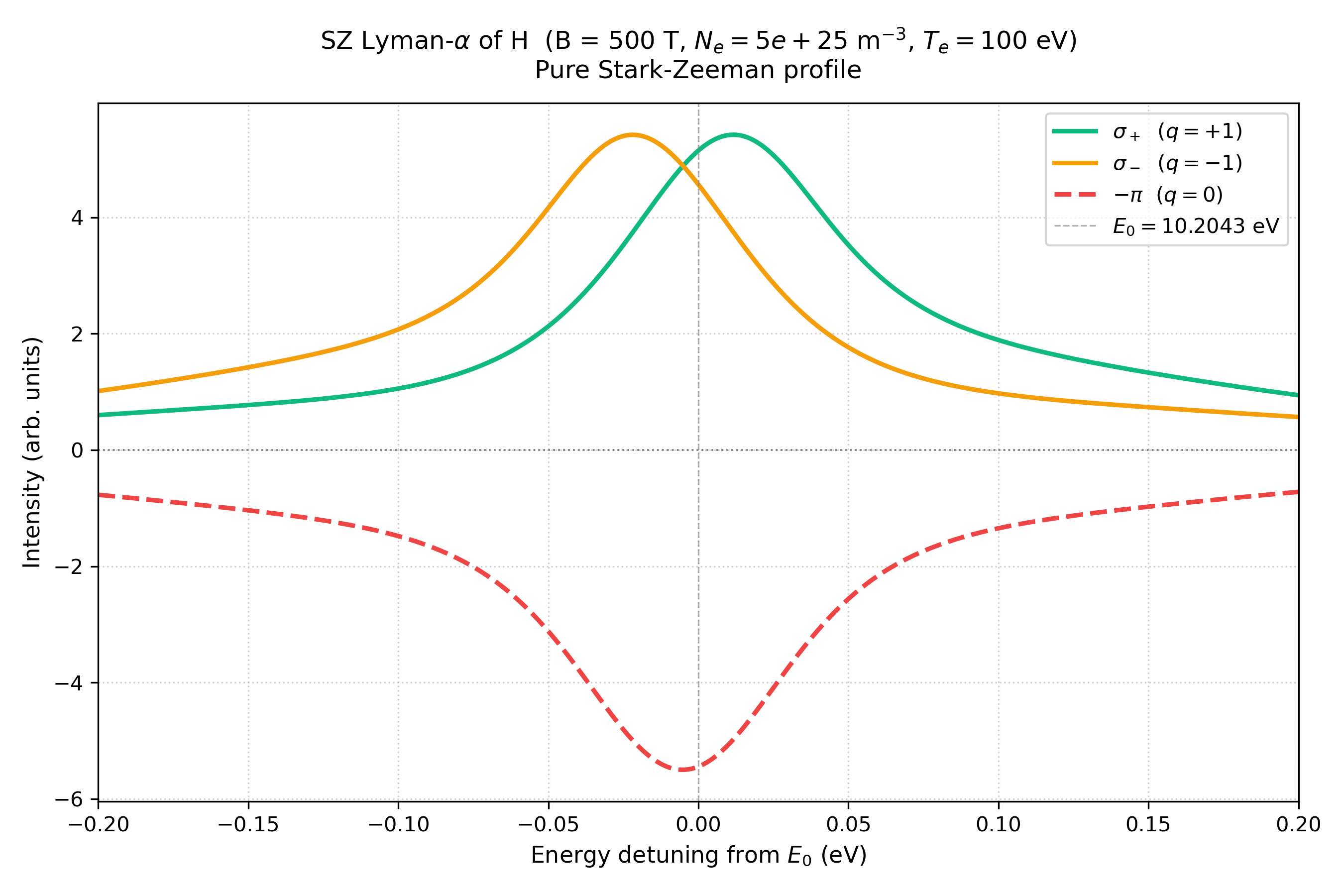
π, σ+, σ− components of H Ly-α at B = 500 T.
B = 1000 T (test_lyman_alpha_1000T.py)
 1#!/usr/bin/env python3
 2"""
 3H Lyman-alpha Stark-Zeeman Splitting at B = 1000 T
 4
 5Highest-field companion to test_lyman_alpha.py / test_lyman_alpha_500T.py,
 6loosely inspired by the Figure 3 benchmark of Ferri, Peyrusse & Calisti
 7(2022, DOI: 10.1063/5.0058552) — that figure used C VI (Z = 6); this script
 8uses H (Z = 1) throughout.
 9
10Conditions:
11  - Radiator: H (Z = 1), Lyman-alpha (n=2 → n=1)
12  - B = 1000 T
13  - Ne = 5e25 m^-3
14  - Te = 100 eV
15  - No convolution (pure Stark-Zeeman profile)
16
17Energy range ±1.0 eV around E0 to accommodate the large Zeeman splitting
18at this extreme field.  The pi component is multiplied by -1 for visual
19separation of polarizations.
20"""
21
22import os
23import sys
24import numpy as np
25import matplotlib.pyplot as plt
26
27sys.path.insert(0, os.path.abspath(os.path.join(os.path.dirname(__file__), "..")))
28
29from starkzee.utils import energy_ev_to_wavelength_nm, RYDBERG_EV
30from starkzee.static_profile import calculate_static_profile
31
32
33def run_test():
34    # ── Physical parameters ────────────────────────────────────────────────
35    Z  = 1        # Hydrogen
36    B  = 1000.0   # Tesla
37    Ne = 5e25     # m^-3
38    Te = 100.0    # eV
39
40    # Unperturbed Lyman-alpha for H (n=2 → n=1)
41    E0 = (Z**2) * RYDBERG_EV * (1.0 - 1.0/4.0)
42
43    # Energy grid: ±1.0 eV around E0
44    detuning_grid = np.linspace(-1.0, 1.0, 800)
45    energies_ev   = E0 + detuning_grid
46
47    print("=" * 70)
48    print("test_lyman_alpha_1000T: H Lyman-alpha — B = 1000 T")
49    print(f"  Z={Z}, B={B} T, Ne={Ne:.1e} m^-3, Te={Te} eV")
50    print(f"  E0 = {E0:.6f} eV  ({energy_ev_to_wavelength_nm(E0):.6f} nm)")
51    print("=" * 70)
52
53    print("-> Computing static Stark-Zeeman profile (unconvolved)…")
54    pi, sig_plus, sig_minus = calculate_static_profile(
55        n_u=2, n_l=1, Z=Z, B=B, Ne_m3=Ne, Te_ev=Te,
56        energies_ev=energies_ev,
57        num_f=30, num_mu=10,
58        use_screening=True,
59        quadratic_zeeman=True,
60        frequency_dependent_width=True,
61    )
62
63    # ── Plot ───────────────────────────────────────────────────────────────
64    fig, ax = plt.subplots(figsize=(9, 6))
65
66    ax.plot(detuning_grid, sig_plus,  color='#10b981', linewidth=2.2,
67            label=r'$\sigma_+$  ($q = +1$)')
68    ax.plot(detuning_grid, sig_minus, color='#f59e0b', linewidth=2.2,
69            label=r'$\sigma_-$  ($q = -1$)')
70    ax.plot(detuning_grid, -pi,       color='#ef4444', linewidth=2.2,
71            linestyle='--', label=r'$-\pi$  ($q = 0$)')
72
73    ax.axhline(0, color='gray', linestyle=':', linewidth=0.9)
74    ax.axvline(0, color='gray', linestyle='--', linewidth=0.8, alpha=0.6,
75               label=f'$E_0 = {E0:.4f}$ eV')
76
77    ax.set_title(
78        f"SZ Lyman-$\\alpha$ of H  (B = {B:.0f} T, "
79        f"$N_e = {Ne:.0e}$ m$^{{-3}}$, $T_e = {Te:.0f}$ eV)\n"
80        r"Pure Stark-Zeeman profile",
81        fontsize=12, pad=12,
82    )
83    ax.set_xlabel(r"Energy detuning from $E_0$ (eV)", fontsize=11)
84    ax.set_ylabel("Intensity (arb. units)", fontsize=11)
85    ax.set_xlim(-1.0, 1.0)
86
87    ax.grid(True, linestyle=':', alpha=0.55)
88    ax.legend(frameon=True, fontsize=10)
89
90    plt.tight_layout()
91    plot_file = os.path.join(os.path.dirname(__file__), "lyman_alpha_1000T.png")
92    plt.savefig(plot_file, dpi=300)
93    print(f"Plot saved → {plot_file}")
94    plt.show()
95
96
97if __name__ == "__main__":
98    run_test()
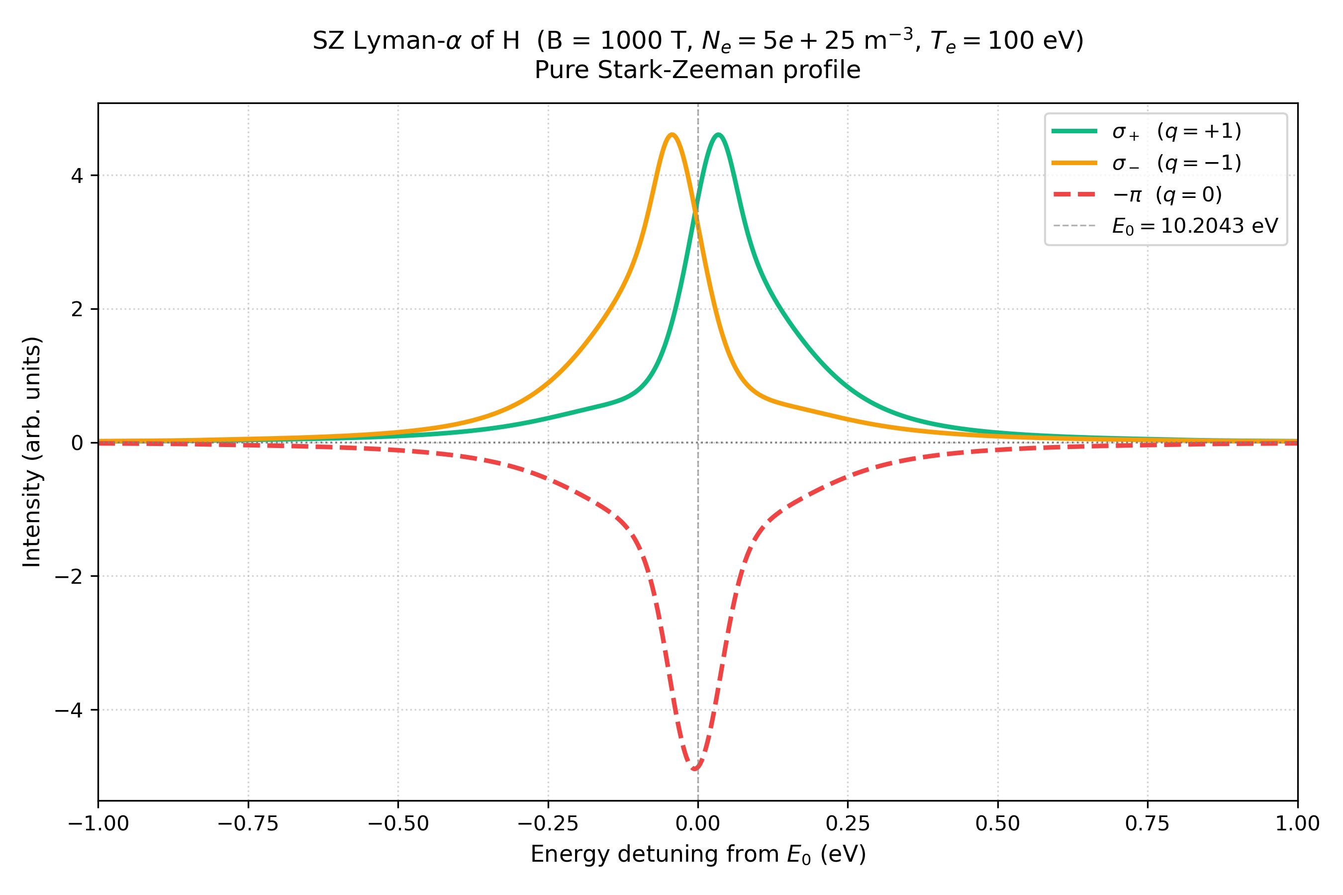
π, σ+, σ− components of H Ly-α at B = 1000 T.