Hα stick spectrum and broadened profile

Script: examples/example_halpha.py

Side-by-side comparison of the discrete transition stick spectrum (discrete_transitions) and the static Stark-Zeeman broadened profile at B = 0, 3, and 10 T, at two electron densities (\(N_e = 10^{17}\) and \(10^{19}\) m^-3), showing the transition from the Zeeman-dominated to the Stark-dominated regime.

Code

"""
example_halpha.py — H Balmer-alpha (n=3→2) Stark-Zeeman profiles.

Shows static profiles for B = 1, 5, 10 T at two electron densities:
  • Ne = 10^20 m^-3 : Zeeman-dominated  (±5 meV window)
  • Ne = 10^23 m^-3 : Stark-dominated   (±30 meV window)
Te = 5 eV throughout.

Run:
    python example_halpha.py

Produces:  example_halpha.png
"""

import numpy as np
import matplotlib.pyplot as plt
import sys, os
sys.path.insert(0, os.path.abspath(os.path.join(os.path.dirname(__file__), "..")))

from starkzee.static_profile import calculate_static_profile, discrete_transitions
from starkzee.utils import reduced_mass_rydberg_ev

# ── Parameters ────────────────────────────────────────────────────────────────

Z, n_u, n_l = 1, 3, 2
A           = 1          # atomic mass (1 = H)
Te_ev       = .5
Ti_ev       = .5
E0 = (Z**2) * reduced_mass_rydberg_ev(Z, A) * (1.0 / n_l**2 - 1.0 / n_u**2)

B_VALS  = [0.0, 3.0, 10.0]        # Tesla
NE_ROWS = [
    (1e17, 1.0),   # (Ne m^-3, detuning half-range meV)
    (1e19, 1.0),
]
NPTS = 500   # Voigt bakes in Doppler; grid only needs to resolve ~Doppler width (~50 ueV)

POL_COLOR = {0: "#e74c3c", -1: "#3498db", 1: "#2ecc71"}

# ── Precompute stick spectra (field-independent per B) ────────────────────────

print("Computing stick spectra …")
sticks = {}
for B in B_VALS:
    sticks[B] = discrete_transitions(
        n_u=n_u, n_l=n_l, Z=Z, B=B,
        fine_structure=True, min_strength=0
    )

# ── Figure ────────────────────────────────────────────────────────────────────

fig, axes = plt.subplots(2, 3, figsize=(14, 8), constrained_layout=True)

for row, (Ne, det_range) in enumerate(NE_ROWS):
    ne_exp   = int(np.log10(Ne))
    det_mev  = np.linspace(-det_range, det_range, NPTS)
    energies = E0 + det_mev * 1e-3

    for col, B in enumerate(B_VALS):
        ax = axes[row, col]

        print(f"  B={B:.0f} T,  Ne=1e{ne_exp} m^-3 ...", flush=True)

        pi, sp, sm = calculate_static_profile(
            n_u=n_u, n_l=n_l, Z=Z, B=B,
            Ne_m3=Ne, Te_ev=Te_ev,
            energies_ev=energies,
            num_f=25, num_mu=8,
            fine_structure=True,
            frequency_dependent_width=True,
            Ti_ev=Ti_ev, species='H',
        )

        # 90° transverse: I = I_π + ½(I_σ+ + I_σ−)
        transverse = pi + 0.5 * (sp + sm)
        norm  = transverse.max() or 1.0

        # Centre detuning on the intensity-weighted centroid so that the
        # fine-structure blueshift does not break the visual σ+/σ− symmetry.
        E_center = float(np.sum(energies * transverse) / np.sum(transverse))
        det_plot = (energies - E_center) * 1e3   # meV from FS line center

        # ── Profile curves ────────────────────────────────────────────────
        ax.fill_between(det_plot, transverse / norm, alpha=0.10, color="k")
        ax.plot(det_plot, transverse / norm, "k",       lw=1.8, label="Transverse")
        ax.plot(det_plot, pi / norm,         color=POL_COLOR[0],
                lw=1.1, ls="--", alpha=0.85, label="π")
        ax.plot(det_plot, 0.5*(sp+sm) / norm, color=POL_COLOR[-1],
                lw=1.1, ls=":",  alpha=0.85, label="½(σ+σ−)")

        # ── Stick spectrum overlay (scaled to 0.45 of plot height) ────────
        tr      = sticks[B]
        det_stk = (tr["energy_ev"] - E_center) * 1e3
        s_stk   = tr["strength"] / tr["strength"].max() * 0.45
        for q in [0, -1, 1]:
            mask = (tr["q"] == q) & (np.abs(det_stk) <= det_range)
            if mask.any():
                ax.vlines(det_stk[mask], 0, s_stk[mask],
                          colors=POL_COLOR[q], alpha=0.35, lw=1.0)
                ax.plot(det_stk[mask], s_stk[mask], '.',
                          color=POL_COLOR[q], alpha=0.35, lw=1.0)

        # ── Axes decoration ───────────────────────────────────────────────
        ax.set_title(
            f"B = {B:.0f} T  |  $N_e = 10^{{{ne_exp}}}$ m$^{{-3}}$",
            fontsize=10
        )
        ax.set_xlabel("Detuning from line center (meV)", fontsize=9)
        ax.set_ylabel("Norm. intensity",                  fontsize=9)
        ax.set_xlim(-det_range, det_range)
        ax.set_ylim(0, 1.15)
        ax.axhline(0, color="grey", lw=0.4)
        ax.tick_params(labelsize=8)

        if row == 0 and col == 0:
            ax.legend(fontsize=8, framealpha=0.75, loc="upper right")

print("Done.  Saving example_halpha.png …")

fig.suptitle(
    f"H Balmer-α  (n=3→2, Z=1)  ·  Static Stark-Zeeman + Doppler  ·"
    f"  $T_e = T_i$ = {Te_ev:.1f} eV",
    fontsize=13
)
plt.savefig("example_halpha.png", dpi=150, bbox_inches="tight")
plt.show()

Result

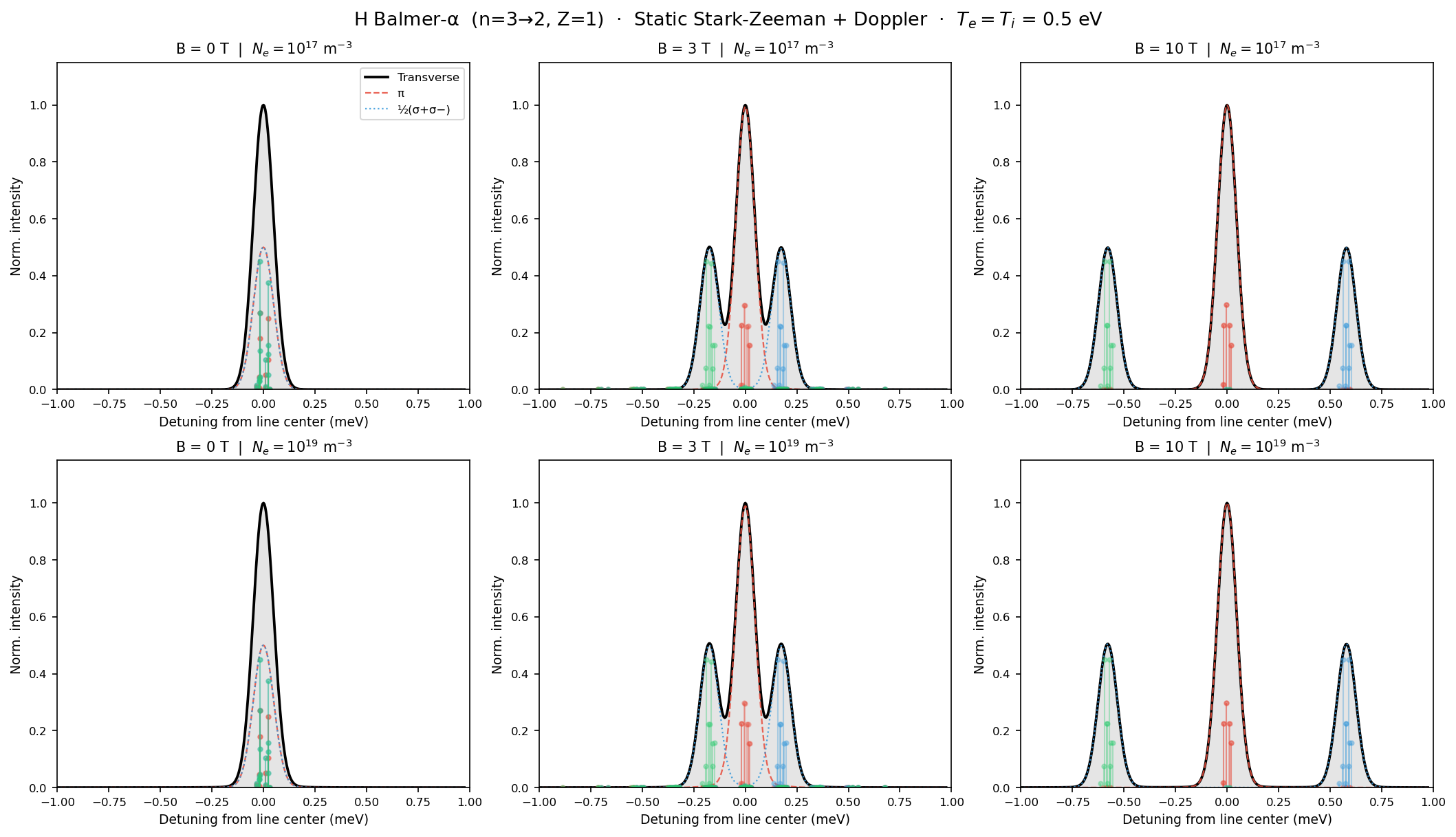
Transverse profile (with π and ½(σ++σ−) components) and the zero-field stick spectrum overlaid, across a grid of B and \(N_e\) values.