Transition anatomy
Script: examples/example_transitions.py
Explores the discrete Stark-Zeeman transitions of H Ly-α (n=2→1) and related lines: prints a transition table with energies, polarizations, and dipole strengths at B = 5 T, prints oscillator strengths and Einstein A coefficients for a set of H lines, and builds a six-panel figure spanning:
Ly-α stick spectrum at B = 0 (fine-structure splitting only)
Ly-α stick spectrum at B = 5 T (Zeeman comparable to fine structure)
Full static profile with the B = 5 T stick spectrum overlaid
How a Stark field splits an otherwise degenerate B = 2 T manifold
Hβ (n=4→2) stick spectrum at B = 5 T — many Stark-Zeeman components
Ly-α at B = 5000 T — the Zeeman-dominated regime (\(\mu_B B \gg \xi\)), completing the story set up by panels 1 and 2
Code
  1"""
  2example_transitions.py — Discrete Stark-Zeeman transitions and full profiles.
  3
  4Demonstrates:
  5  1. Listing individual transitions and their line strengths
  6  2. Stick spectra at B=0 and B=5T side by side (pure Zeeman)
  7  3. Full static profile with stick spectrum overlay
  8  4. Oscillator strengths and Einstein A coefficients for common lines
  9  5. Stark + Zeeman: how a microfield splits an otherwise degenerate manifold
 10
 11Run:
 12    python example_transitions.py
 13
 14Produces:  example_transitions.png
 15"""
 16
 17import numpy as np
 18import matplotlib.pyplot as plt
 19import matplotlib.gridspec as gridspec
 20import sys, os
 21sys.path.insert(0, os.path.abspath(os.path.join(os.path.dirname(__file__), "..")))
 22
 23from starkzee.static_profile import discrete_transitions, calculate_static_profile
 24from starkzee.radiator import line_strength, oscillator_strength, einstein_a
 25from starkzee.utils import reduced_mass_rydberg_ev, energy_ev_to_wavelength_nm
 26
 27# ─────────────────────────────────────────────────────────────────────────────
 28# Helpers
 29# ─────────────────────────────────────────────────────────────────────────────
 30
 31POL_COLOR = {0: "#e74c3c", -1: "#3498db", 1: "#2ecc71"}  # π, σ+, σ−
 32POL_LABEL = {0: "π (q=0)", -1: "σ+ (q=−1)", 1: "σ− (q=+1)"}
 33
 34
 35def bohr_energy(n_u, n_l, Z, A=1):
 36    return (Z**2) * reduced_mass_rydberg_ev(Z, A) * (1.0/n_l**2 - 1.0/n_u**2)
 37
 38
 39def plot_stick_spectrum(ax, tr, E0, normalize=True, title="", show_legend=True):
 40    """Plot discrete transitions as vertical lines colored by polarization."""
 41    det = (tr['energy_ev'] - E0) * 1e3  # detuning in meV
 42    s = tr['strength']
 43    if normalize and s.max() > 0:
 44        s = s / s.max()
 45    for q in [0, -1, 1]:
 46        mask = tr['q'] == q
 47        if mask.any():
 48            ax.vlines(det[mask], 0, s[mask],
 49                      colors=POL_COLOR[q], label=POL_LABEL[q],
 50                      linewidth=1.8, alpha=0.85)
 51    ax.set_xlabel("Detuning from E₀ (meV)", fontsize=10)
 52    ax.set_ylabel("Norm. strength" if normalize else "|d|² (a₀²)", fontsize=10)
 53    ax.set_title(title, fontsize=11)
 54    if show_legend:
 55        ax.legend(fontsize=8, framealpha=0.7)
 56    ax.axhline(0, color="grey", linewidth=0.5)
 57    ax.set_xlim(-5, 5)
 58
 59
 60# ─────────────────────────────────────────────────────────────────────────────
 61# 1. Print transition table for H Ly-α at B=5T
 62# ─────────────────────────────────────────────────────────────────────────────
 63
 64print("=" * 65)
 65print("H Ly-α (n=2→1, Z=1) discrete transitions at B=5 T")
 66print("=" * 65)
 67Z, n_u, n_l, B = 1, 2, 1, 5.0
 68E0 = bohr_energy(n_u, n_l, Z)
 69
 70tr = discrete_transitions(n_u=n_u, n_l=n_l, Z=Z, B=B,
 71                           fine_structure=True, min_strength=1e-6)
 72
 73print(f"{'#':>3}  {'E (eV)':>12}  {'ΔE (meV)':>10}  {'q':>4}  "
 74      f"{'|d|² (a₀²)':>12}  {'upper':>6}  {'lower':>6}")
 75print("-" * 65)
 76for k in range(len(tr['energy_ev'])):
 77    det_mev = (tr['energy_ev'][k] - E0) * 1e3
 78    pol = {0: "π", -1: "σ+", 1: "σ−"}[tr['q'][k]]
 79    print(f"{k+1:>3}  {tr['energy_ev'][k]:>12.6f}  {det_mev:>10.4f}  "
 80          f"{pol:>4}  {tr['strength'][k]:>12.6f}  "
 81          f"{tr['upper_idx'][k]:>6}  {tr['lower_idx'][k]:>6}")
 82
 83S_ul = line_strength(n_u, n_l, Z)
 84print(f"\nSum of strengths : {tr['strength'].sum():.6f} a₀²")
 85print(f"line_strength()  : {S_ul:.6f} a₀²  (must match)")
 86
 87
 88# ─────────────────────────────────────────────────────────────────────────────
 89# 2. Atomic data table
 90# ─────────────────────────────────────────────────────────────────────────────
 91
 92print("\n" + "=" * 65)
 93print("Oscillator strengths and Einstein A coefficients")
 94print("=" * 65)
 95LINES = [
 96    ("H  Ly-α", 2, 1, 1),
 97    ("H  Ly-β", 3, 1, 1),
 98    ("H  Ly-γ", 4, 1, 1),
 99    ("H  Hα  ", 3, 2, 1),
100    ("H  Hβ  ", 4, 2, 1),
101    ("H  Hγ  ", 5, 2, 1),
102]
103print(f"{'Line':>12}  {'gf':>8}  {'S_ul (a₀²)':>12}  {'A_ul (s⁻¹)':>14}")
104print("-" * 52)
105for name, nu, nl, Zl in LINES:
106    gf  = oscillator_strength(nu, nl, Zl)
107    S   = line_strength(nu, nl, Zl)
108    A   = einstein_a(nu, nl, Zl)
109    print(f"{name:>12}  {gf:>8.4f}  {S:>12.4f}  {A:>14.4e}")
110
111
112# ─────────────────────────────────────────────────────────────────────────────
113# 3. Build figure
114# ─────────────────────────────────────────────────────────────────────────────
115
116fig = plt.figure(figsize=(10, 9))
117gs = gridspec.GridSpec(2, 3, figure=fig, hspace=0.45, wspace=0.38)
118
119ax_b0   = fig.add_subplot(gs[0, 0])
120ax_b5   = fig.add_subplot(gs[0, 1])
121ax_full = fig.add_subplot(gs[0, 2])
122ax_stark = fig.add_subplot(gs[1, 0])
123ax_hb   = fig.add_subplot(gs[1, 1])
124ax_hib  = fig.add_subplot(gs[1, 2])
125
126# ── Panel 1: H Ly-α stick at B=0 ────────────────────────────────────────────
127tr_b0 = discrete_transitions(n_u=2, n_l=1, Z=1, B=0.0,
128                               fine_structure=True, min_strength=1e-6)
129plot_stick_spectrum(ax_b0, tr_b0, E0,
130                    title="H Ly-α  B=0 T\n(SO splits 2p₁/₂ from 2p₃/₂)")
131
132# ── Panel 2: H Ly-α stick at B=5T ───────────────────────────────────────────
133tr_b5 = discrete_transitions(n_u=2, n_l=1, Z=1, B=5.0,
134                               fine_structure=True, min_strength=1e-6)
135plot_stick_spectrum(ax_b5, tr_b5, E0,
136                    title="H Ly-α  B=5 T\n(Zeeman + SO)")
137
138# ── Panel 3: Full static profile overlaid with sticks ───────────────────────
139Ne, Te = 1e23, 5.0
140energies = E0 + np.linspace(-0.005, 0.005, 1000)
141pi, sp, sm = calculate_static_profile(
142    n_u=2, n_l=1, Z=1, B=5.0, Ne_m3=Ne, Te_ev=Te,
143    energies_ev=energies, num_f=25, num_mu=8,
144    fine_structure=True, frequency_dependent_width=False
145)
146det_ev  = (energies - E0) * 1e3
147total   = pi + sp + sm
148total_n = total / total.max()
149
150ax_full.plot(det_ev, total_n, color="k", linewidth=1.5, label="Total profile")
151ax_full.plot(det_ev, pi / total.max(), color=POL_COLOR[0],
152             linewidth=1.0, linestyle="--", alpha=0.7, label="π")
153ax_full.plot(det_ev, (sp + sm) / total.max(), color=POL_COLOR[-1],
154             linewidth=1.0, linestyle=":", alpha=0.7, label="σ+σ−")
155
156# Overlay sticks (normalized to profile peak)
157s5 = tr_b5['strength']
158s5_n = s5 / s5.max() * 0.5
159det5 = (tr_b5['energy_ev'] - E0) * 1e3
160for q in [0, -1, 1]:
161    mask = tr_b5['q'] == q
162    ax_full.vlines(det5[mask], 0, s5_n[mask],
163                   colors=POL_COLOR[q], alpha=0.4, linewidth=1.2)
164
165ax_full.set_xlabel("Detuning (meV)", fontsize=10)
166ax_full.set_ylabel("Norm. intensity", fontsize=10)
167ax_full.set_title(f"H Ly-α  B=5 T  Ne={Ne:.0e} m⁻³\nProfile + stick spectrum",
168                  fontsize=11)
169ax_full.set_xlim(-5, 5)
170ax_full.legend(fontsize=8, framealpha=0.7)
171
172# ── Panel 4: Stark + Zeeman — how a microfield splits lines ─────────────────
173B_panel = 2.0
174E0_lya = bohr_energy(2, 1, 1)
175for Fz_vm, alpha in [(0.0, 1.0), (5e7, 0.65), (2e8, 0.35)]:
176    tr_f = discrete_transitions(n_u=2, n_l=1, Z=1, B=B_panel,
177                                 Fz=Fz_vm, fine_structure=False,
178                                 min_strength=1e-6)
179    det = (tr_f['energy_ev'] - E0_lya) * 1e3
180    s   = tr_f['strength'] / tr_f['strength'].max()
181    label = f"F={Fz_vm:.0e} V/m" if Fz_vm > 0 else "F=0"
182    ax_stark.vlines(det, 0, s * alpha, alpha=alpha,
183                    colors=["#7f8c8d", "#e67e22", "#8e44ad"][
184                        [0.0, 5e7, 2e8].index(Fz_vm)],
185                    linewidth=1.5, label=label)
186
187ax_stark.set_xlabel("Detuning (meV)", fontsize=10)
188ax_stark.set_ylabel("Norm. strength", fontsize=10)
189ax_stark.set_title(f"H Ly-α  B={B_panel} T + Stark field\n"
190                   f"(sticks: all polarizations combined)", fontsize=11)
191ax_stark.legend(fontsize=8, framealpha=0.7)
192ax_stark.set_xlim(-8, 8)
193ax_stark.axhline(0, color="grey", linewidth=0.5)
194
195# ── Panel 5: H Hβ stick at B=5T ─────────────────────────────────────────────
196E0_hb = bohr_energy(4, 2, 1)
197tr_hb = discrete_transitions(n_u=4, n_l=2, Z=1, B=5.0,
198                               fine_structure=True, min_strength=1e-5)
199det_hb = (tr_hb['energy_ev'] - E0_hb) * 1e3
200s_hb   = tr_hb['strength'] / tr_hb['strength'].max()
201for q in [0, -1, 1]:
202    mask = tr_hb['q'] == q
203    if mask.any():
204        ax_hb.vlines(det_hb[mask], 0, s_hb[mask],
205                     colors=POL_COLOR[q], linewidth=1.2, alpha=0.85,
206                     label=POL_LABEL[q])
207ax_hb.set_xlabel("Detuning (meV)", fontsize=10)
208ax_hb.set_ylabel("Norm. strength", fontsize=10)
209ax_hb.set_title("H Hβ (n=4→2)  B=5 T\nMany Stark-Zeeman components", fontsize=11)
210ax_hb.legend(fontsize=8, framealpha=0.7)
211ax_hb.set_xlim(-12, 12)
212ax_hb.axhline(0, color="grey", linewidth=0.5)
213
214# ── Panel 6: H Ly-α stick at B=5000T — Zeeman dominates over SO ─────────────
215# Complements Panels 1 (B=0, pure SO) and 2 (B=5T, SO and Zeeman comparable):
216# at very high B the Zeeman splitting (∝ B) overtakes the fixed SO splitting,
217# so the pattern below is dominated by the linear-in-B Zeeman structure.
218B_hib = 5000.0
219tr_hib = discrete_transitions(n_u=2, n_l=1, Z=1, B=B_hib,
220                               fine_structure=True, min_strength=1e-6)
221det_hib = (tr_hib['energy_ev'] - E0) * 1e3
222s_hib   = tr_hib['strength'] / tr_hib['strength'].max()
223for q in [0, -1, 1]:
224    mask = tr_hib['q'] == q
225    if mask.any():
226        ax_hib.vlines(det_hib[mask], 0, s_hib[mask],
227                      colors=POL_COLOR[q], linewidth=1.8, alpha=0.85,
228                      label=POL_LABEL[q])
229ax_hib.set_xlabel("Detuning from E₀ (meV)", fontsize=10)
230ax_hib.set_ylabel("Norm. strength", fontsize=10)
231ax_hib.set_title(f"H Ly-α  B={B_hib:.0f} T\nZeeman dominates (μ_B B ≫ ξ)", fontsize=11)
232ax_hib.legend(fontsize=8, framealpha=0.7)
233ax_hib.axhline(0, color="grey", linewidth=0.5)
234
235fig.suptitle("starkzee — Discrete Stark-Zeeman Transitions", fontsize=14, y=1.01)
236plt.tight_layout()
237out = os.path.join(os.path.dirname(__file__), "example_transitions.png")
238plt.savefig(out, dpi=150, bbox_inches="tight")
239print(f"Saved {out}")
240plt.show()
Result
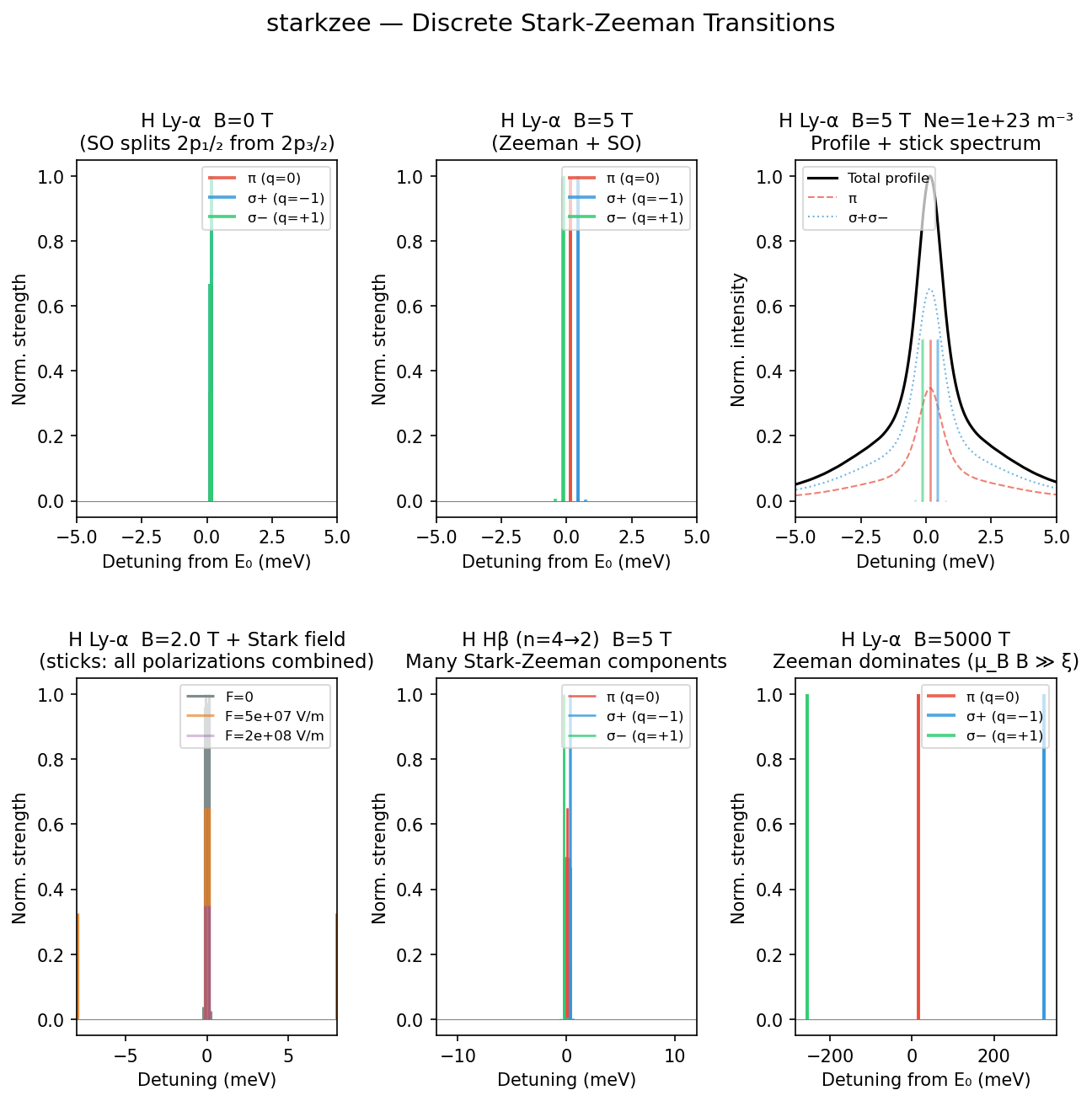
From pure fine-structure splitting (B = 0) through Zeeman-comparable (B = 5 T) to Zeeman-dominated (B = 5000 T) regimes, plus Stark mixing and the denser Hβ manifold.