StarkZee vs. built-in reference models

Script: examples/model_comparison.py

Compares StarkZee’s static and FFM (dynamic-ion) solvers against all five built-in reference models (Voigt, Stehlé, Stehlé-parameterized, Rosato; here Lomanowski is disabled since it has no magnetic-field treatment) for D-α (n=3→2) at \(N_e = 10^{20}\) m^-3, \(T_i = T_e = 1\) eV, \(B = 3\) T, \(\theta = 90^\circ\). Uses use_empirical_data=True so both StarkZee solvers land on the measured NIST line center (see Empirical Field-Free Energies) for a fair comparison against the reference models, which are anchored to their own tabulated NIST air wavelength. Can save the figure to a file when given a path on the command line, which is how the figure at the end of the Built-in Reference Models page was produced (the same figure is shown below).

Code

"""
model_comparison.py — Compare StarkZee's static and FFM profiles against
analytical and tabulated models.

Edit the parameters block inside run() to change plasma conditions.
All models receive the same (Ti, Te, Ne, B, angle), so differences are
purely due to the underlying physics model.

Run directly::

    python examples/model_comparison.py                 # show interactively
    python examples/model_comparison.py out/figure.png  # save to file
"""

import time
import traceback

import numpy as np
import matplotlib.pyplot as plt

from starkzee.line_profile import LineProfile
from starkzee.convolutions import calculate_doppler_width_ev
import starkzee.models as models


def run(save_path=None):
    # ── parameters ────────────────────────────────────────────────────────────
    n_u, n_l       = 3, 2      # transition  (Hα)
    species        = 'D'       # emitting species: 'H', 'D', or 'T'
    Ne_m3          = 1e20      # electron density          [m⁻³]
    Te_ev          = 1       # electron temperature      [eV]  → Stark width
    Ti_ev          = 1       # ion temperature           [eV]  → Doppler width
    B              = 3.0       # magnetic field            [T]
    view_angle_deg = 90.0      # observation angle to B    [deg]
    # ──────────────────────────────────────────────────────────────────────────

    # Line center and adaptive grid width
    lp = LineProfile(n_u=n_u, n_l=n_l, B=B, Ne_m3=Ne_m3, Te_ev=Te_ev, Ti_ev=Ti_ev,
                     species=species, view_angle_deg=view_angle_deg)

    delta_E_D        = calculate_doppler_width_ev(lp.E0, Ti_ev, A_emitter=1)
    delta_lambda_D_nm = lp.E0_wavelength_nm * delta_E_D / lp.E0
    half_width_nm    = max(2.1, 4.0 * delta_lambda_D_nm)

    # StarkZee computes in vacuum nm, on a grid centered on the gross-structure
    # Rydberg line center.  Compute it up front so the comparison models can be
    # referenced to its actual line center (next).
    wl_sz_nm = np.linspace(lp.E0_wavelength_nm - half_width_nm,
                            lp.E0_wavelength_nm + half_width_nm, 3000)
    print('--------\ntimings:\n--------')
    t0 = time.time()
    lp.compute_static_profile(wl_sz_nm, grid_type='wavelength_nm',  num_f=60, num_mu=11, use_empirical_data=True, atom=species)
    print(f'starkzee (static): {time.time() - t0:.3g} sec')

    # StarkZee FFM (dynamic ion) profile, on the same vacuum-nm grid and
    # plasma parameters; Doppler broadening is applied internally by the FFM
    # solver (apply_doppler=True default), so both curves are directly
    # comparable.
    lp_ffm = LineProfile(n_u=n_u, n_l=n_l, B=B, Ne_m3=Ne_m3, Te_ev=Te_ev, Ti_ev=Ti_ev,
                         species=species, view_angle_deg=view_angle_deg)
    t0 = time.time()
    lp_ffm.compute_ffm_profile(wl_sz_nm, grid_type='wavelength_nm', sdt_bin_tol=1e-5, use_empirical_data=True, atom=species)
    print(f'starkzee (ffm): {time.time() - t0:.3g} sec')
    ffm_profile = lp_ffm.profile

    # Physical line center = intensity-weighted centroid of the StarkZee profile.
    # With use_empirical_data the levels carry the Lamb shift, so the centroid
    # falls on the physical (NIST) wavelength.  The comparison models have
    # no fine structure and are symmetric about their grid mean, so centering their
    # grid and the vertical guide line on this centroid makes every peak overlay;
    # otherwise StarkZee appears offset from the others and from the vertical line.
    #center_air_nm = lp.E0_wavelength_air_nm
    center_air_nm = float(np.sum(lp.wavelengths_air_nm * lp.profile) / np.sum(lp.profile))

    # Comparison models compute in air nm, centered on the same physical line center.
    wl_cmp_nm = np.linspace(center_air_nm - half_width_nm,
                             center_air_nm + half_width_nm, 5000)

    # ── figure ────────────────────────────────────────────────────────────────
    fig, (ax1, ax2) = plt.subplots(1, 2, figsize=[12, 5])
    fig.suptitle(
        f'$n_e = {Ne_m3:.2g}$ m$^{{-3}}$,  '
        f'$T_i = {Ti_ev:.3g}$ eV,  $T_e = {Te_ev:.3g}$ eV\n'
        f'$B = {B:.3g}$ T,  $\\theta = {view_angle_deg:.3g}$°'
    )

    # ── comparison models ─────────────────────────────────────────────
    cmp_funcs = {
        'voigt':        models.voigt,
        'stehle':       models.stehle,
        'stehle_param': models.stehle_param,
        #'lomanowski':   models.lomanowski,
        'rosato':   models.rosato,
    }

    for name, func in cmp_funcs.items():
        try:
            t0 = time.time()
            profile = func(
                wl_cmp_nm, n_u, n_l, B, Ne_m3, Te_ev, Ti_ev,
                view_angle_deg=view_angle_deg, species=species,
            )
            print(f'{name}: {time.time() - t0:.3g} sec')
            ax1.plot(wl_cmp_nm, profile / profile.max(), label=name)
            ax2.plot(wl_cmp_nm, profile / profile.max(), label=name)
        except Exception as exc:
            print(f'{name} failed: {exc}')
            traceback.print_exc()

    # ── StarkZee static and FFM profiles (computed above) ─────────────────────
    y = lp.profile / lp.profile.max()
    y_ffm = ffm_profile / ffm_profile.max()
    for ax in (ax1, ax2):
        ax.plot(lp.wavelengths_air_nm, y, 'k--', linewidth=2, label='starkzee (static)')
        ax.plot(lp_ffm.wavelengths_air_nm, y_ffm, 'k:', linewidth=2, label='starkzee (ffm)')

    # ── formatting ────────────────────────────────────────────────────────────
    for ax in (ax1, ax2):
        ax.set_xlim(wl_cmp_nm.min(), wl_cmp_nm.max())
        ax.axvline(center_air_nm, ls='--', color='dimgrey', zorder=0)
        ax.legend(fontsize=10)
        ax.set_xlabel('wavelength (nm)', fontsize=10)

    ax1.set_xlim(center_air_nm - 0.2, center_air_nm + 0.2)
    ax2.set_xlim(center_air_nm - 2, center_air_nm + 2)
    ax2.semilogy()
    plt.tight_layout()

    if save_path:
        fig.savefig(save_path, dpi=200)
        print(f'saved figure to {save_path}')
    else:
        plt.show()


if __name__ == '__main__':
    import sys
    run(save_path=sys.argv[1] if len(sys.argv) > 1 else None)

Result

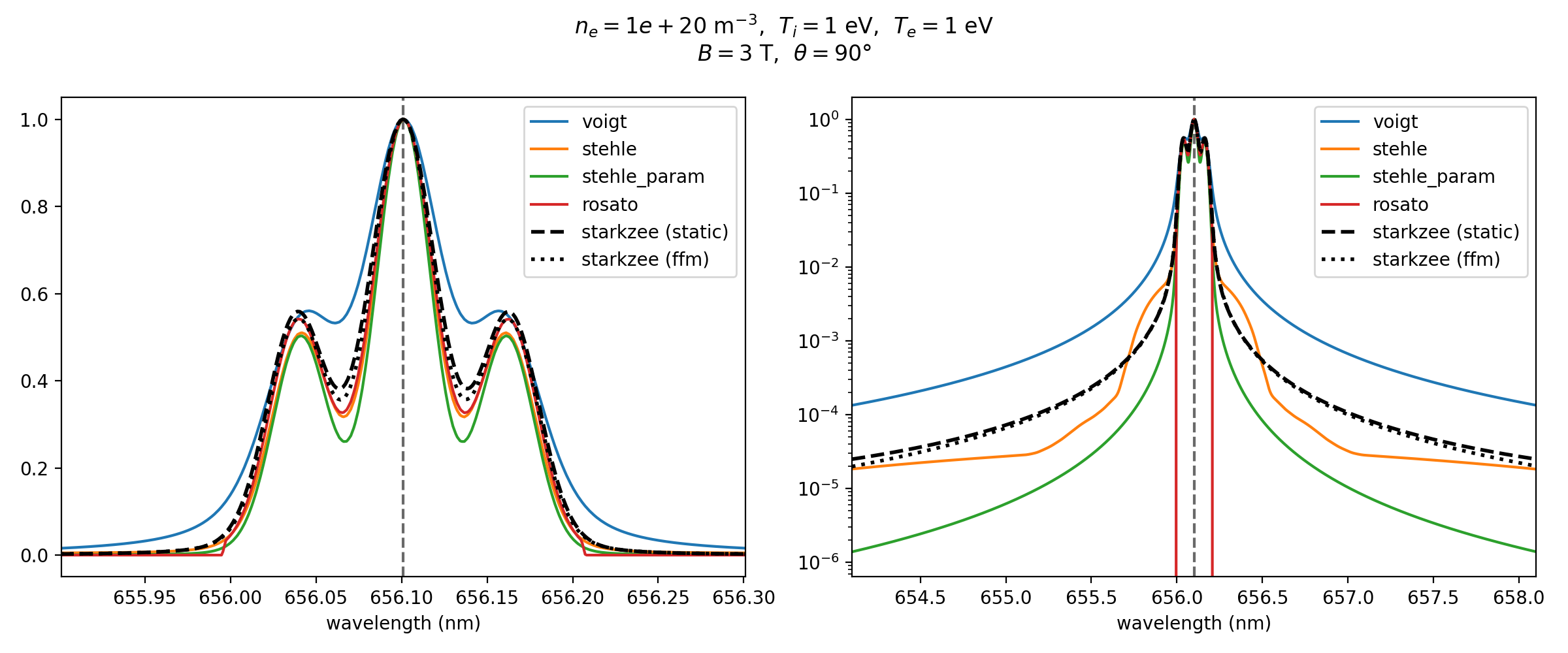
StarkZee (static and FFM) against the field-treating (Rosato) and field-free (Voigt, Stehlé, Stehlé-parameterized) reference models. Linear scale (left) and log scale (right).