Reproducing Figure 1 from Ferri et al. (2022)

A script computing the full Balmer-series (Hα–Hε) Stark-Zeeman spectrum for H, in the style of Figure 1 of Ferri, Peyrusse & Calisti (2022), at B = 100, 500, 1000 T, comparing the profile with and without the quadratic Zeeman term in the Hamiltonian. All five lines are summed on one common wavelength grid (Case B recombination weighting) so the individual line wings overlap into a single continuous spectrum.

Note

This script is a qualitative illustration, not a quantitative reproduction of Ferri et al. Fig. 1. Ferri et al. build a configuration-interaction Hamiltonian mixing states of different principal quantum numbers, and note this inter-\(n\) mixing is crucial for the quadratic Zeeman term at these field strengths. StarkZee currently diagonalizes the quadratic Zeeman (and Stark) Hamiltonian within a single principal shell only (see Approximations and Numerical Choices); each Balmer line here is computed independently and the results are overlaid. In particular, the inter-\(n\)-driven red shift of the high-PQN lines (Hβ, Hδ) that Ferri Fig. 1(c) shows at B = 1 kT is not reproduced — StarkZee’s intra-shell treatment shifts these lines blue instead. See TODO item 1 for the underlying analysis.

Full Balmer series (reproduce_fig1.py)

#!/usr/bin/env python3
"""
reproduce_fig1.py
==================
Full Balmer-series (H-alpha ... H-epsilon) Stark-Zeeman spectrum for H, in
the style of Ferri, Peyrusse & Calisti (2022) Fig. 1.

All five lines are computed on one common wavelength grid spanning the whole
Balmer range, so their Stark-broadened wings overlap into a single continuous
spectrum rather than five disconnected local windows.  Each line is weighted
by its Case B recombination intensity relative to H-beta, divided by its
oscillator strength, so the integrated flux of each transition reproduces
the Case B Balmer decrement.

Conditions (Ferri, Peyrusse & Calisti 2022, Fig. 1):
  Z = 1, Ne = 1e23 m^-3, Te = 5 eV, transverse observation.

Three B values (100, 500, 1000 T) are shown, each with and without the
quadratic Zeeman term in the Hamiltonian.
"""

import os, sys
import numpy as np
import matplotlib.pyplot as plt
sys.path.insert(0, os.path.abspath(os.path.join(os.path.dirname(__file__), "..")))

from starkzee.utils import wavelength_nm_to_energy_ev
from starkzee.static_profile import calculate_static_profile
from starkzee.radiator import line_strength


# ---------------------------------------------------------------------------
# Balmer line definitions
# ---------------------------------------------------------------------------
BALMER_LINES = [
    (3, "Hα", r"H$\alpha$",   6563),
    (4, "Hβ", r"H$\beta$",    4861),
    (5, "Hγ", r"H$\gamma$",   4340),
    (6, "Hδ", r"H$\delta$",   4102),
    (7, "Hε", r"H$\epsilon$", 3970),
]

# Standard Case B recombination relative intensities (relative to H-beta = 1)
# (Osterbrock & Ferland 2006, T ~ 10,000 K, ne -> 0, optically thick Lyman series).
_CASEB = {3: 2.86, 4: 1.00, 5: 0.47, 6: 0.26, 7: 0.16}


def balmer_spectrum(B, Ne, Te, Ti, wavelengths_nm, quadratic_zeeman):
    """Case-B-weighted transverse intensity summed over Halpha-Hepsilon on a
    single common wavelength grid, so the individual line wings overlap into
    one continuous spectrum instead of disconnected local windows."""
    energies = wavelength_nm_to_energy_ev(wavelengths_nm)
    total = np.zeros_like(energies)
    for n_u, name_ascii, _, _ in BALMER_LINES:
        print(f"    {name_ascii} (n={n_u}->2) ...", end=" ", flush=True)
        S_n = line_strength(n_u, n_l=2, Z=1)
        weight = _CASEB[n_u] / S_n   # integral of weight * profile dE -> _CASEB[n_u]
        pi, sp, sm = calculate_static_profile(
            n_u=n_u, n_l=2, Z=1, B=B, Ne_m3=Ne, Te_ev=Te,
            energies_ev=energies,
            num_f=20, num_mu=6,
            use_screening=True,
            quadratic_zeeman=quadratic_zeeman,
            frequency_dependent_width=False,
            Ti_ev=Ti,
        )
        total += weight * (pi + 0.5 * (sp + sm))
        print("done.")
    return total


# ---------------------------------------------------------------------------
if __name__ == "__main__":
    Ne, Te = 1e23, 5.0
    Ti = Te  # ion temperature not separately specified; assume Ti = Te
    B_list = [100.0, 500.0, 1000.0]

    wavelengths_nm  = np.linspace(380.0, 720.0, 3000)
    wavelengths_ang = wavelengths_nm * 10.0

    print("reproduce_fig1: full Balmer-series Stark-Zeeman spectrum")
    print(f"  Ne = {Ne:.1e} m-3, Te = {Te} eV, Z = 1")
    print()

    spectra = {}
    for B in B_list:
        print(f"B = {int(B)} T:")
        print("  Without quadratic Zeeman:")
        nq = balmer_spectrum(B, Ne, Te, Ti, wavelengths_nm, quadratic_zeeman=False)
        print("  With    quadratic Zeeman:")
        yq = balmer_spectrum(B, Ne, Te, Ti, wavelengths_nm, quadratic_zeeman=True)
        spectra[B] = (nq, yq)
        print()

    print("All done. Plotting ...")

    # ── Figure layout: 3 rows (one per B), full Balmer range per panel ───────
    fig, axes = plt.subplots(3, 1, figsize=(11, 10), sharex=True)
    fig.suptitle(
        rf"Full Balmer series (H$\alpha$-H$\epsilon$)  |  H, "
        rf"$N_e={Ne:.0e}$ m$^{{-3}}$, $T_e={Te:.0f}$ eV"
        "\n"
        r"Solid = with quadratic Zeeman, Dashed = without",
        fontsize=13)

    colors = ["tab:blue", "tab:orange", "tab:red"]
    B_labels = [f"B = {int(B)} T" for B in B_list]

    for ax, B, label, color in zip(axes, B_list, B_labels, colors):
        nq, yq = spectra[B]
        peak = max(yq.max(), nq.max(), 1.0)

        ax.plot(wavelengths_ang, nq / peak, "--", color=color,
                lw=1.2, alpha=0.75, label=f"{label}  (no QZ)")
        ax.plot(wavelengths_ang, yq / peak, "-",  color=color,
                lw=1.6, label=f"{label}  (with QZ)")

        for _, _, _, wl in BALMER_LINES:
            ax.axvline(wl, color="gray", lw=0.6, ls=":", alpha=0.5)

        ax.set_yscale("log")
        ax.set_ylim(1e-5, 3.0)
        ax.set_ylabel("Norm. intensity", fontsize=10)
        ax.legend(loc=4, fontsize=9)
        ax.grid(True, which="both", alpha=0.3)

    for _, _, name_tex, wl in BALMER_LINES:
        axes[0].text(wl, 1.0, name_tex, ha="center", va="bottom", fontsize=9,
                     bbox=dict(facecolor="white", alpha=0.7, pad=1, edgecolor="none"))

    axes[-1].set_xlabel(r"Wavelength ($\AA$)", fontsize=12)
    axes[-1].set_xlim(wavelengths_ang.min(), wavelengths_ang.max())

    plt.tight_layout()
    out = os.path.join(os.path.dirname(__file__), "reproduce_fig1.png")
    plt.savefig(out, dpi=200, bbox_inches="tight")
    print(f"Saved plot to {out}")
    plt.show()

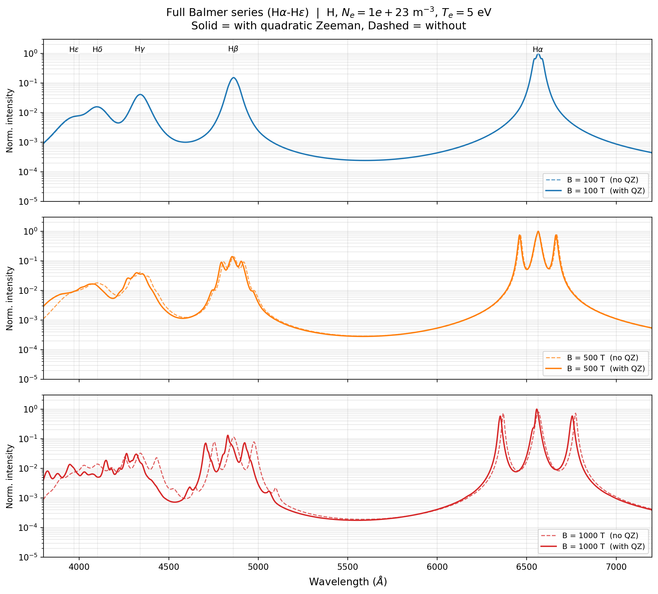
Hα–Hε summed on a common grid (Case B weighting) at B = 100, 500, 1000 T, solid = with quadratic Zeeman, dashed = without.