Quadratic Zeeman polarization wings

Script: examples/reproduce_halpha_wings.py

Demonstrates the polarization-wing effect at B = 500 T and B = 1000 T: at high field the quadratic Zeeman term shifts the 3p(\(m_l=\pm1\)) → 2s transitions away from the main Hα cluster, creating distinct shoulders/wings in the σ± components that only appear when quadratic_zeeman=True. A modest ion temperature (Ti_ev=Te) is used so the underlying Stark-Zeeman components — narrower than natural linewidth at this low density — are resolved on the plotted grid rather than undersampled.

Code

#!/usr/bin/env python3
"""
reproduce_halpha_wings.py
=========================
Focused examination of Hα (n=3→2, Z=1) σ+, σ−, π polarization components
at B = 500 T and B = 1000 T, comparing with and without the quadratic
(diamagnetic) Zeeman term.

Physical picture
----------------
Without QZ all σ+ (or all σ−) Hα transitions are degenerate at
  E_σ+ = E0 + μ_B·B     (all Δml=+1 components)
  E_σ− = E0 − μ_B·B

With QZ the diagonal shift of each |n,l,ml⟩ state is
  ΔE_QZ = (e²B²/8mₑ) · ⟨r²⟩_nl · ⟨sin²θ⟩_{l,ml}

For n=3 the relevant shifts (B=1000 T):
  3p, ml=±1: +8.87 meV   ← LARGEST in n=3
  3s, ml=0 : +8.50 meV
  3d, ml=±2: +6.65 meV
  3d, ml=±1: +4.43 meV
  3d, ml=0 : +3.69 meV

For n=2:
  2s, ml=0 : +1.72 meV
  2p, ml=±1: +1.48 meV
  2p, ml=0 : +0.74 meV

The dominant oscillator-strength contributor is 3d→2p (radial dipole ≈4.75 a₀).
The 3p→2s transitions (radial dipole ≈3.06 a₀, oscillator fraction ~21 %)
have LARGER n=3 QZ shifts, so they appear as a separate shoulder:

  σ+ wing: 3p(ml=+1) → 2s(ml=0)   at E0 + μ_B·B + (8.87−1.72) = E0+μ_B·B+7.1 meV
  σ− wing: 3p(ml=−1) → 2s(ml=0)   at E0 − μ_B·B + (8.87−1.72) = E0−μ_B·B+7.1 meV
            → this is ~7 meV NEARER to E0 than the main 3d cluster

These wings are ONLY present with quadratic_zeeman=True.
"""

import numpy as np
import matplotlib.pyplot as plt
import sys, os
sys.path.insert(0, os.path.abspath(os.path.join(os.path.dirname(__file__), "..")))

from starkzee.static_profile import calculate_static_profile
from starkzee.utils import reduced_mass_rydberg_ev, BOHR_MAGNETON_EV_T

# ── parameters ───────────────────────────────────────────────────────────────
Z, n_u, n_l = 1, 3, 2
Ne, Te      = 1e17, 5.0
E0          = (Z**2) * reduced_mass_rydberg_ev(Z, 1) * (1.0/n_l**2 - 1.0/n_u**2)

# Fine energy grid — wide enough to cover both σ± at B=1000 T
DET_HALF = 0.10          # ±100 meV
NPTS     = 4000
det      = np.linspace(-DET_HALF, DET_HALF, NPTS)   # eV
energies = E0 + det

# ── compute profiles ─────────────────────────────────────────────────────────
results = {}
for B in [500.0, 1000.0]:
    print(f"  B={int(B)} T: without QZ …", end=" ", flush=True)
    pi_nq, sp_nq, sm_nq = calculate_static_profile(
        n_u, n_l, Z, B, Ne, Te, energies,
        num_f=30, num_mu=8,
        use_screening=True, quadratic_zeeman=False,
        frequency_dependent_width=False, Ti_ev=Te)
    print("done.  With QZ …", end=" ", flush=True)
    pi_yq, sp_yq, sm_yq = calculate_static_profile(
        n_u, n_l, Z, B, Ne, Te, energies,
        num_f=30, num_mu=8,
        use_screening=True, quadratic_zeeman=True,
        frequency_dependent_width=False, Ti_ev=Te)
    print("done.")
    results[B] = dict(
        pi_nq=pi_nq, sp_nq=sp_nq, sm_nq=sm_nq,
        pi_yq=pi_yq, sp_yq=sp_yq, sm_yq=sm_yq,
    )

# ── plot ─────────────────────────────────────────────────────────────────────
det_meV = det * 1e3   # meV axis

fig, axes = plt.subplots(2, 3, figsize=(15, 9), sharey='row')
fig.suptitle(
    r"H$\alpha$ (n=3→2, Z=1) polarization wings from quadratic Zeeman"
    "\n"
    r"$N_e = 10^{17}$ m$^{-3}$, $T_e = 5$ eV — solid: with QZ, dashed: without QZ",
    fontsize=12)

pol_labels = [r"$\pi$", r"$\sigma^+$", r"$\sigma^-$"]
pol_keys   = [("pi_nq", "pi_yq"), ("sp_nq", "sp_yq"), ("sm_nq", "sm_yq")]
pol_colors = ["tab:blue", "tab:red", "tab:green"]

for row, B in enumerate([500.0, 1000.0]):
    r = results[B]
    zeeman_meV = BOHR_MAGNETON_EV_T * B * 1e3

    # Expected wing positions (meV from E0)
    # QZ shifts at this B (all scale as B²):
    coeff = (1.60218e-19 * B**2 * (5.29177e-11)**2 / (8 * 9.10938e-31)) * 1e3  # meV
    qz_3p_pm1 = coeff * 180 * 4/5      # n=3,l=1,ml=±1: r2=180, sin2=4/5
    qz_3d_ml2 = coeff * 126 * 6/7      # n=3,l=2,ml=±2: r2=126, sin2=6/7
    qz_2s     = coeff * 42  * 2/3      # n=2,l=0,ml=0
    qz_2p_pm1 = coeff * 30  * 4/5      # n=2,l=1,ml=±1

    wing_sigp_meV  = zeeman_meV + (qz_3p_pm1 - qz_2s)
    wing_sigm_meV  = -zeeman_meV + (qz_3p_pm1 - qz_2s)
    main_sigp_meV  = zeeman_meV + (qz_3d_ml2 - qz_2p_pm1)
    main_sigm_meV  = -zeeman_meV + (qz_3d_ml2 - qz_2p_pm1)

    for col, (label, (nq_key, yq_key), color) in enumerate(
            zip(pol_labels, pol_keys, pol_colors)):
        ax = axes[row, col]
        nq = r[nq_key]
        yq = r[yq_key]
        peak = max(yq.max(), nq.max(), 1e-20)

        ax.plot(det_meV, nq / peak, 'k--', lw=1.2, alpha=0.8, label='No QZ')
        ax.plot(det_meV, yq / peak, color=color, lw=1.8, label='With QZ')

        # Annotate expected wing positions
        if col == 1:  # σ+
            ax.axvline(wing_sigp_meV, color='orange', ls=':', lw=1.2,
                       label=f'3p(ml=+1)→2s wing\n({wing_sigp_meV:.1f} meV)')
            ax.axvline(main_sigp_meV, color='gray',   ls=':', lw=1.0,
                       label=f'3d cluster edge\n({main_sigp_meV:.1f} meV)')
        if col == 2:  # σ−
            ax.axvline(wing_sigm_meV, color='orange', ls=':', lw=1.2,
                       label=f'3p(ml=−1)→2s wing\n({wing_sigm_meV:.1f} meV)')
            ax.axvline(main_sigm_meV, color='gray',   ls=':', lw=1.0,
                       label=f'3d cluster edge\n({main_sigm_meV:.1f} meV)')

        ax.set_xlabel('Detuning from $E_0$ (meV)', fontsize=10)
        ax.set_ylabel('Normalized intensity', fontsize=9)
        ax.set_title(f'B = {int(B)} T — {label}', fontsize=11)
        ax.legend(fontsize=7.5, loc='upper right')
        ax.grid(True, alpha=0.25)
        ax.set_xlim(-100, 100)
        ax.set_ylim(-0.02, None)

plt.tight_layout()
out = "halpha_wings.png"
plt.savefig(out, dpi=200, bbox_inches='tight')
print(f"\nSaved {out}")
plt.show()

Result

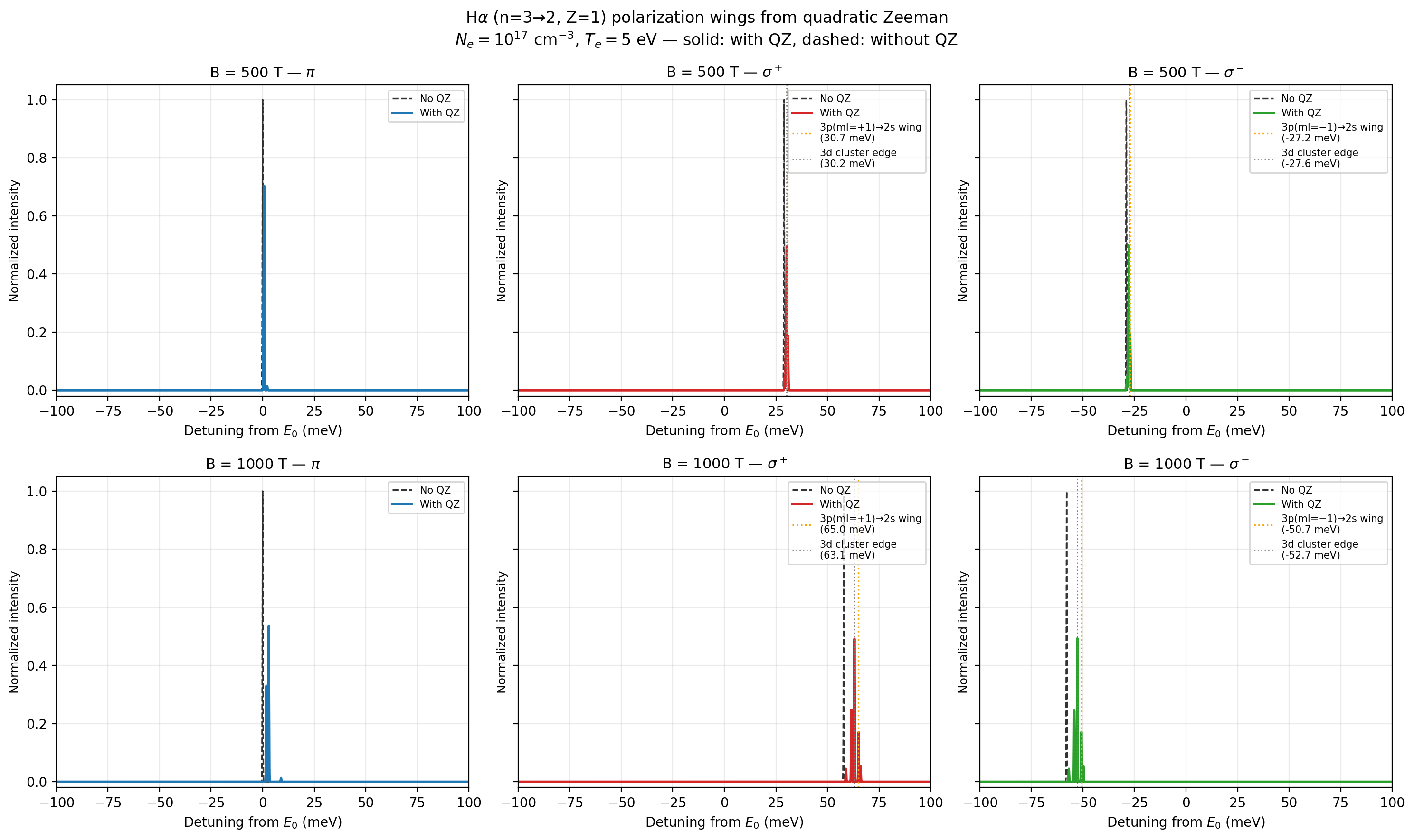
π, σ+, σ− components at B = 500 T and B = 1000 T; solid = with quadratic Zeeman, dashed = without. The 3p→2s wing is resolved as a distinct shoulder at B = 1000 T.